Context
I wanted to test why doubling compute resources does not automatically halve runtime, using repeatable measurements and inspectable raw data.
Approach
I split the midpoint-rule calculation into independent ranges. Worker processes form partial sums, then the parent adds them. I compare end-to-end ProcessPool time against separate sequential references and observe peak RSS.
System
- Midpoint integration for π: 4 / (1 + x²) over [0, 1].
- Pure Python loop without NumPy; processes return partial sums.
- ProcessPoolExecutor with 1, 2, 4, 6, 8 or 12 workers; five runs, median plus minimum and maximum.
- Fixed N for strong scaling, calibrated sizes in a separate block; end-to-end wall time and peak RSS.
- Numerical method
- Worker processes
- Task distribution
- Reduction
- Measurement analysis
Engineering decisions
- Deterministic integration, not Monte Carlo.
- Processes rather than threads for the CPU-bound Python loop; no thread comparison.
- Separate sequential baselines; median and min/max across five repetitions.
What did not work
One CPU-bound algorithm on one system with its scheduler; no CPU affinity. RSS may double-count shared pages. P × T_P is not energy or CPU-time measurement; separate runs can vary.
Result
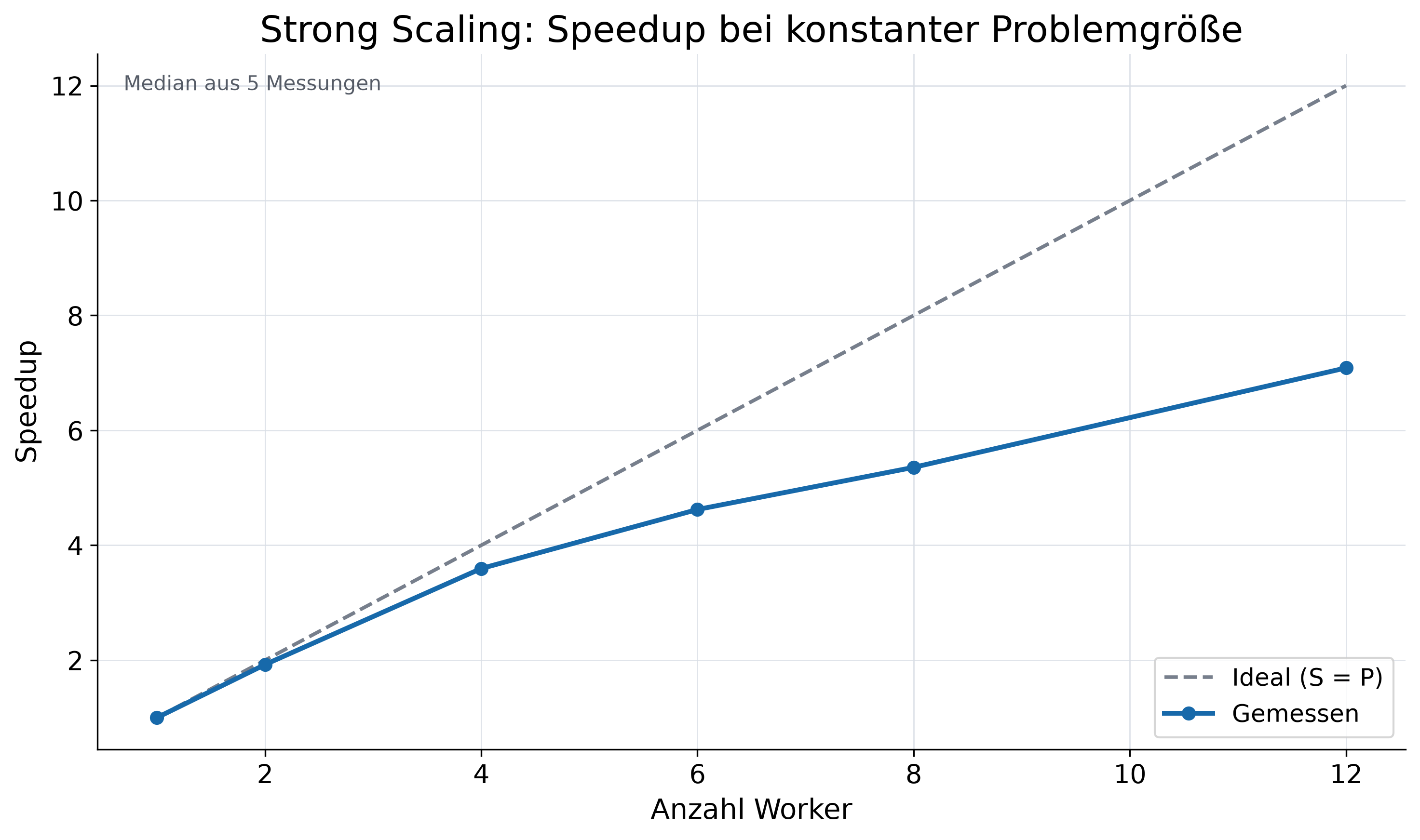
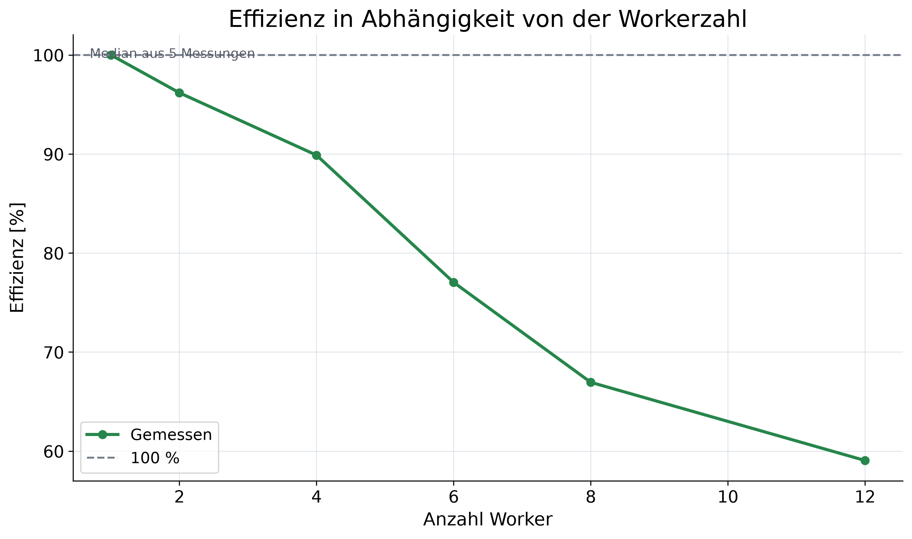
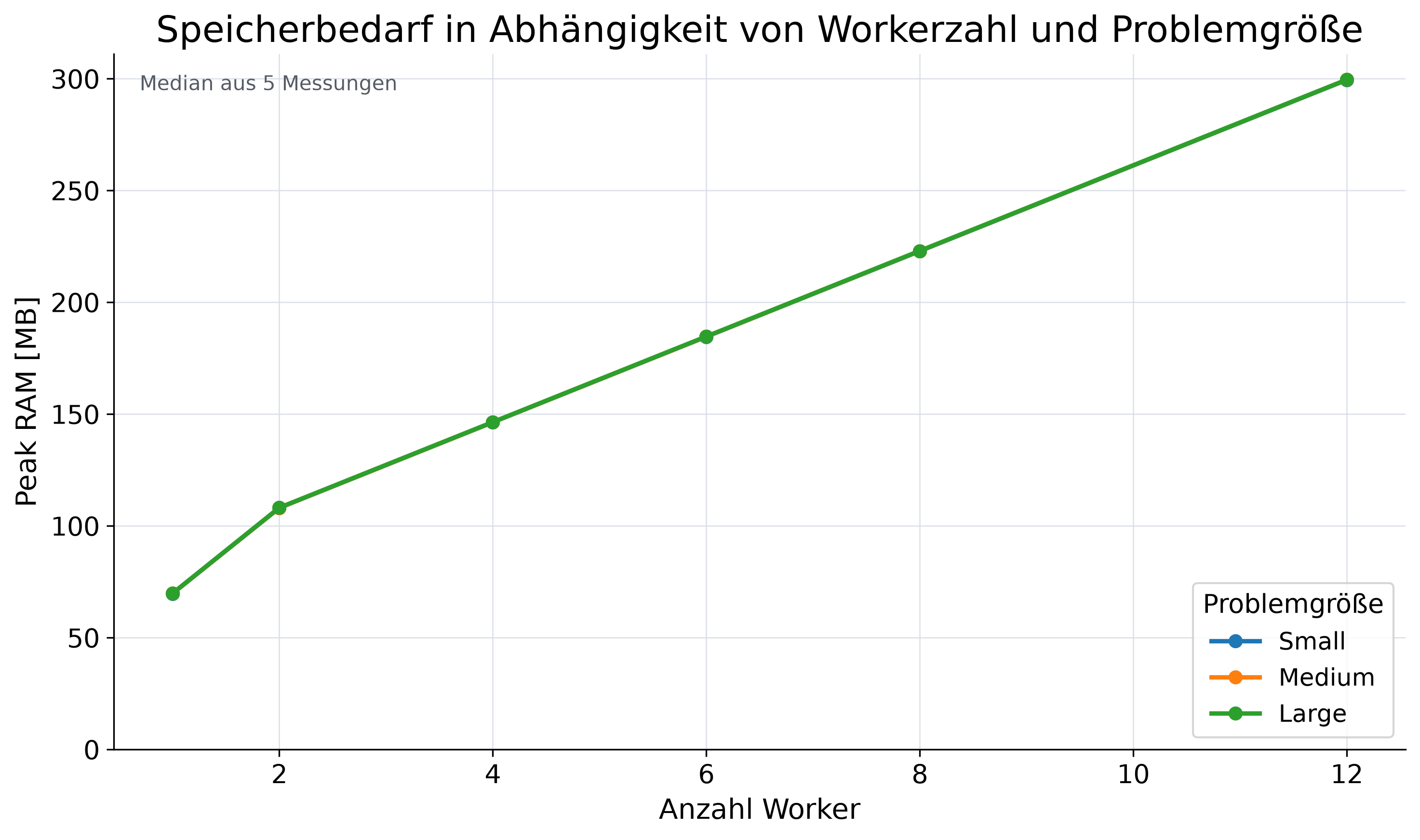
Strong-scaling Large: 4.056 s sequential, 0.572 s with twelve processes (7.09 speedup; about 59% efficiency). P × T_P rises from 4.06 to 6.87 processor-seconds. In the separate size block, peak RSS grows from roughly 70 to 299 MB.
What stayed with me
Parallelism speeds up the calculation, but speedup, efficiency and memory do not scale alike. Useful parallelism depends on whether saved time is worth the management, memory and added resources.
My contribution
The repository contains the benchmark code, the configuration used, raw data, summarized results and the generated figures. The measurements in this case study come from the full run on September 26, 2026.
The question behind the experiment
When two people divide a task, we often imagine they will finish about twice as fast. The same idea seems natural for processors: why not keep adding cores and share every calculation across more of them?
I wanted to know not just whether parallel code was faster, but what overhead remained between splitting the work and producing a result.
Parallel work still has to be combined
A sequential algorithm performs its steps one after another. A parallel algorithm assigns independent subtasks to multiple compute units. For a sum, for example, (a + b) and (c + d) can be calculated at the same time; the two partial results are added afterwards. That final combination is a reduction. It is simple, but it does not disappear just because the earlier work ran in parallel.
That is the first trade-off: some work can happen simultaneously, while other steps still depend on previous results or need coordination. Lecture material on parallel algorithms makes this visible with problems such as sums and prefix sums.[3] A sum worked well for my experiment because each worker could process a disjoint range and return one partial result.
What I measure
Runtime T tells me how long a calculation takes. Speedup compares direct sequential time T_seq with parallel time T_P: S = T_seq / T_P. If eight seconds become two, S = 4. The tested version completes the same work in a quarter of the wall-clock time.
Efficiency relates that speedup to P, the number of worker processes: E = S / P. It does not tell me how busy the CPUs were. It tells me how much speedup I received per process I used. Efficiency is therefore a scaling measure, not a CPU-utilization meter.
For parallel costs I use P × T_P. In this simple model, that expresses how many processor-seconds are associated with P concurrently provisioned compute units over runtime T_P. Management, scheduling, communication, result transfer and reduction are overhead. Memory is another measure: a run can finish sooner and still use more RAM.
Why I calculated π
I chose numerical integration, not a Monte Carlo method. The mathematical starting point is ∫₀¹ 4 / (1 + x²) dx = π: an antiderivative of 1 / (1 + x²) is arctan(x); from zero to one that gives π/4, and multiplying by four gives π.[1]
For the midpoint rule, I divide [0, 1] into N equal intervals, evaluate the function at each midpoint and multiply the sum by the interval width. The loop adds each contribution directly to a running sum instead of storing millions of values.
The intervals are independent. I can split N into contiguous ranges, calculate each range separately and add the partial sums at the end. The mathematical task stays the same; only the order and number of simultaneously executed steps change.
How the benchmark is set up
The benchmark is a pure Python loop without NumPy vectorization. Parallel variants use `concurrent.futures.ProcessPoolExecutor`, which executes tasks in separate processes.[2] Python threads are not part of this comparison.
I test 1, 2, 4, 6, 8 and 12 processes. Each configuration runs five times. The median is the main value; minimum and maximum form the observed range in the runtime charts. ProcessPool time is end-to-end: it includes process management, task distribution, calculation, returning results, reduction and pool shutdown. That is deliberately more than timing only the inner loop.
For memory, `psutil` samples the RSS of the parent process and its child processes about every 15 milliseconds. RSS is the resident memory the operating system associates with a process. It is an approximation, not an exact count of physical RAM pages exclusively occupied by the program.
Three problem sizes, two measurement blocks
Small, Medium and Large are not arbitrary labels. The full run calibrates N automatically against sequential runtime targets. The resulting values were 3,771,022 intervals for Small, 18,997,300 for Medium and 75,392,548 for Large. Their sequential median runtimes in the problem-size experiment were about 0.234 s, 1.170 s and 4.763 s.
It is important not to mix the Large reference from this block with strong scaling. Strong scaling had its own sequential baseline of 4.056 s. The problem-size and strong-scaling tests were separate runs, and each keeps its own reference time. Five repetitions and a median do not make measurements immutable: background load, temperature and scheduling can still change between runs.
Result 1: much faster, but not twelve times
In strong scaling, N stays fixed at 75,392,548. The direct sequential reference is 4.056 s. With two worker processes, the median falls to 2.108 s (speedup 1.92); with four, 1.128 s (3.60); with six, 0.877 s (4.62); with eight, 0.757 s (5.36); and with twelve, 0.572 s (7.09).
Twelve processes make the calculation noticeably faster. But the curve does not reach the ideal twelve. The dashed line in the chart shows S = P: the case where speedup grows in direct proportion to process count. The measured curve stays below it. That gap is not a surprise; it is where non-parallel work and the costs of parallelizing become visible.
Result 2: efficiency declines
Efficiency in the strong-scaling block is about 96 percent with two processes, 90 percent with four, 77 percent with six and 67 percent with eight. At twelve processes it is roughly 59 percent. The calculation keeps getting faster, but every additional process contributes proportionally less speedup than the early ones did.
Those 59 percent do not mean 59 percent CPU utilization. Efficiency here is speedup divided by process count. CPU utilization is a different measure, and I did not measure it in this experiment.
Finishing sooner does not mean using fewer compute resources
In the same strong-scaling block, parallel costs P × T_P rise from about 4.06 processor-seconds at the sequential reference to about 6.87 with twelve processes. The answer arrives much earlier, but this simple cost measure counts more concurrently provisioned compute units over that runtime.
This is neither an energy measurement nor actual process CPU time. It is a theoretical comparison measure that makes the trade-off tangible: shorter waiting time can come with higher total parallel costs.
Result 3: larger tasks benefit more
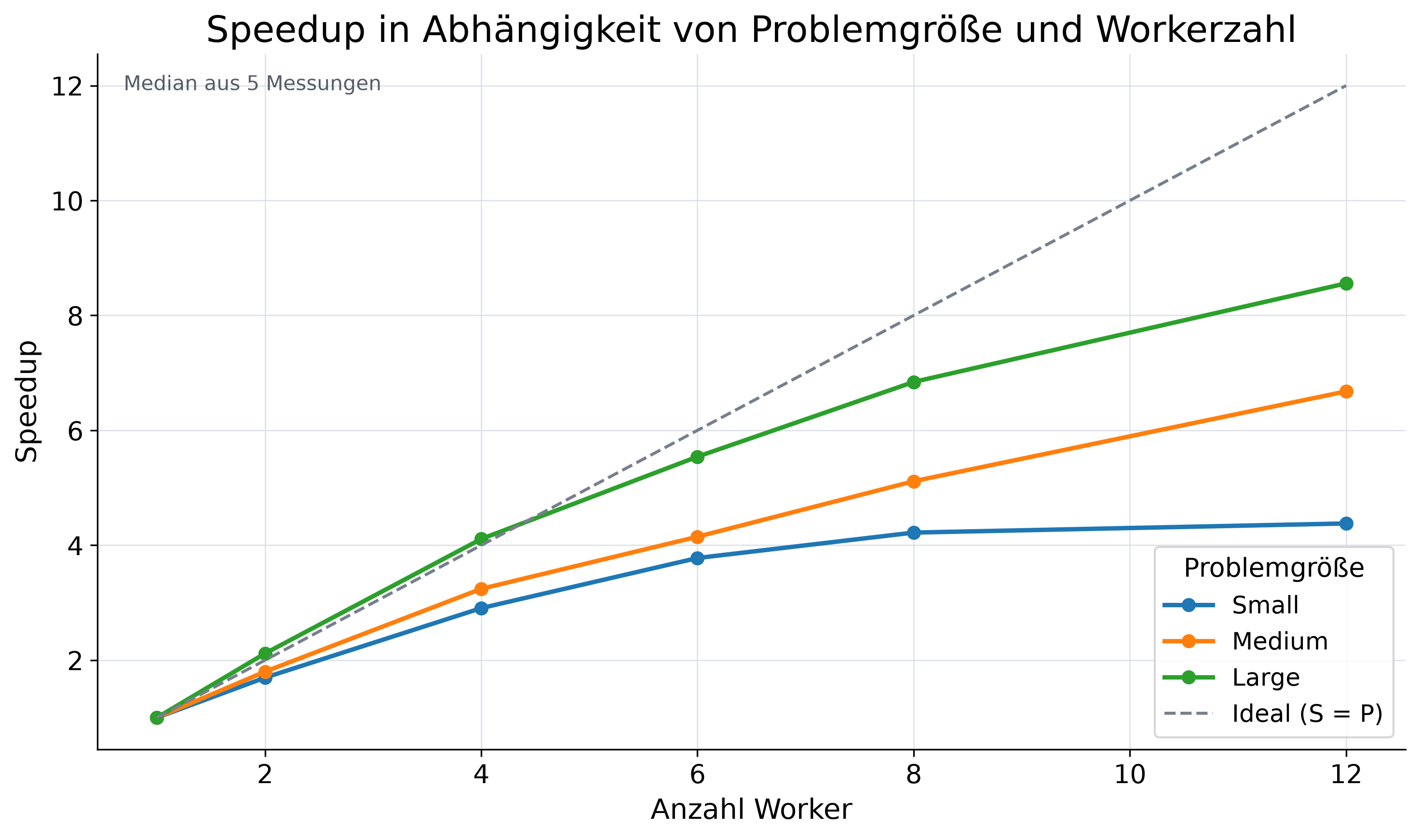
In the separate problem-size experiment, twelve processes reach a speedup of 4.38 for Small, 6.68 for Medium and 8.56 for Large. Each value uses the direct sequential baseline for that same problem size. These speedups are not mixed with the strong-scaling curve.
One plausible explanation is that actual computation makes up a larger share of a bigger task, so one-time management and distribution overhead matters relatively less. That is an interpretation, not a single cause proven in isolation by this experiment. What was measured is the difference across these three sizes under these conditions.
Result 4: memory follows a different curve
Observed peak RSS in the problem-size experiment is about 70 MB for the sequential runs. With twelve processes, Small, Medium and Large each use roughly 299–300 MB. At a given process count, the three problem sizes almost overlap in the chart.
That fits the implementation: N mainly determines how many times the calculation runs. Intermediate values are not stored in a large collection; each process computes one value and adds it immediately to its local sum. A larger N therefore mainly increases runtime here, while the extra memory comes mostly from additional Python processes, their runtime environments and management data.
RSS remains an operating-system approximation. Shared pages, such as libraries, may appear more than once in the summed process values. The curve shows observed peak RSS according to the benchmark’s sampling method, not the exact amount of exclusively occupied RAM.
Result 5: task size changes runtime
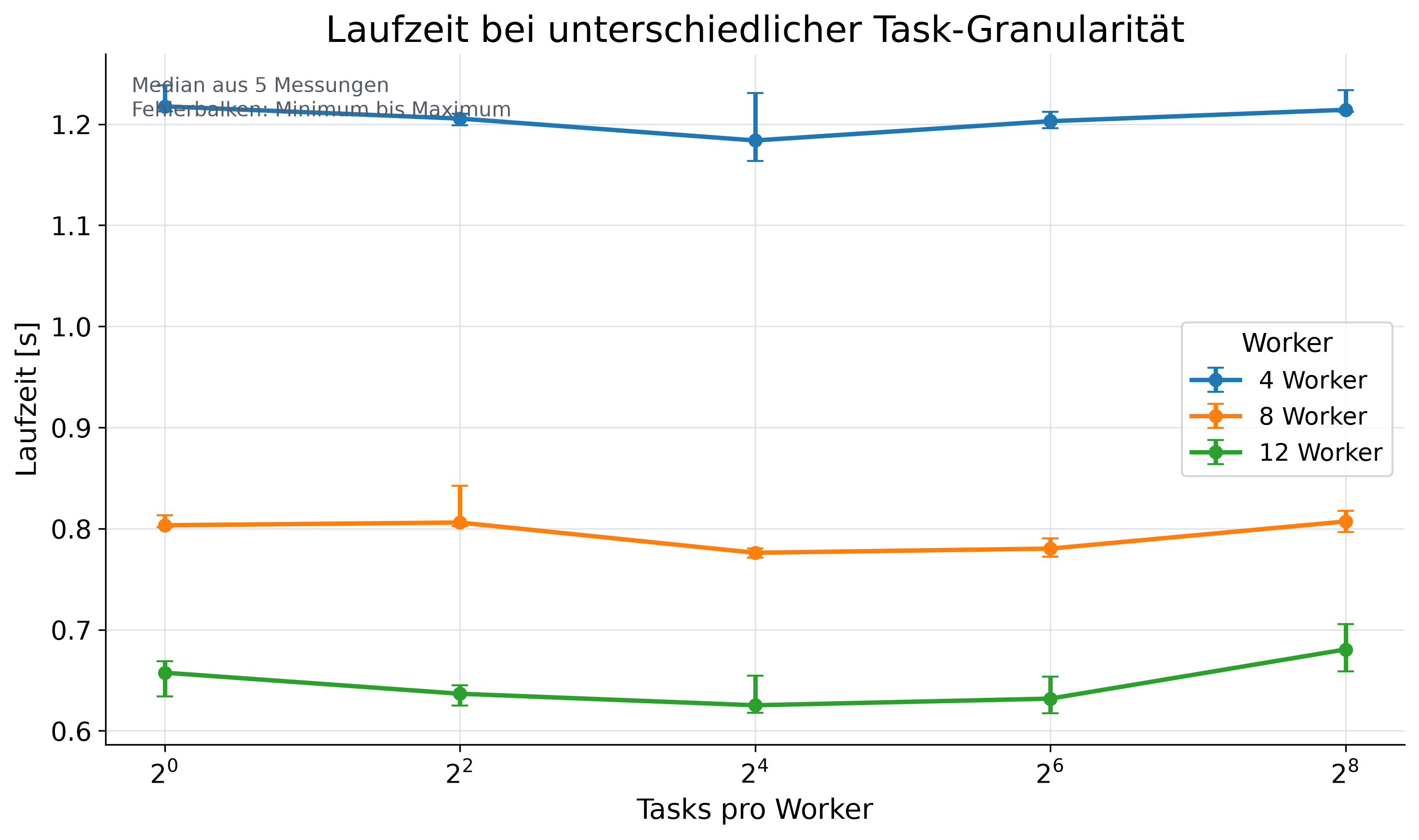
The granularity experiment keeps total work fixed and changes the number of tasks per worker: 1, 4, 16, 64 or 256. With twelve processes, median runtimes are 0.657 s, 0.637 s, 0.625 s, 0.632 s and 0.680 s.
In this run, 16 tasks per process was a little faster than the coarsest and finest splits. Some subdivision can distribute independent ranges more flexibly. Very small tasks add scheduling and management work; very large ones may make balancing coarser. This does not make 16 a universal optimum – it only shows task size was measurable in this benchmark.
What I take away from the experiment
Before the experiment, “more cores” mostly sounded like simple arithmetic to me: divide the work, calculate simultaneously, save time. The measurements confirm the important part – the Large calculation became much faster. But they also show what that simple picture leaves out: speedup stayed below process count, efficiency fell, the RSS estimate rose, and even task splitting changed the result.
The more useful question is not “How many processes can I start?” but “How much parallelism makes sense for this particular task?” I need to consider runtime, management, memory and benefit together. To me, parallelization is not a free speed multiplier; it is an engineering trade-off.
Limits of the experiment
The result applies first to one CPU-heavy numerical integration in pure Python using ProcessPoolExecutor – not automatically to every algorithm or programming language. The full run records an Intel Core Ultra 5 125H with Linux and Python 3.14.4 as its test system. CPU affinity was not enforced; the OS scheduler and changing system load remain part of the conditions.
RSS is a sampled approximation and may count shared memory pages more than once. P × T_P is a theoretical cost measure, not energy or a direct CPU-time measurement. The separate measurement blocks also varied, so I use each series’ own sequential baseline. This does not fully answer the broader question of why chipmakers do not add cores without limit: I did not investigate manufacturing, die area, energy efficiency or economics. My benchmark only examines what software gains from additional parallelism.
Sources and code
The measurements, raw data, configuration and figures come from my own repository. The links below support the short background on parallel algorithms, the midpoint rule and Python process pools.